Previously, we explored the approach of using vector regions to implement the field of view of a turret. Troops approached the turret on open field and no hindrances lay between them. Now suppose there is a hinderance, say a wall, that obscures the visibility of troop from turret; how should we implment that? This tutorial suggest an approach to tackle this issue.
Final Result Preview
Let's take a look at the final result we will be working towards. Click on the turret at the bottom of the stage to start the simulation.
Step 1: The Basic Concept
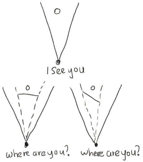
So here's what we try to achieve in this tutorial. Observe the image above. The turret can see the trooper unit if it's within turret's field of view (top). Once we place a wall in between the turret and the trooper, the trooper's visibility is shielded from turret.
Step 2: Recap
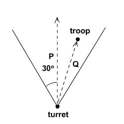
First of all, let's do a little revision. Say the vector of turret's line of sight is P and the vector from turret to trooper is Q. The trooper is visible to the turret if:
- Angle between P and Q is less than the angle of view (in this case 30° on both sides)
- Magnitude of P is more than Q
Step 3: Approach Overview
Above is the pseudo-code for the approach we shall undertake. Determining whether the trooper is within the turret's field of view (FOV) is explained in Step 2. Now let's get to determining whether the trooper is behind a wall.
We shall use vector operations to achieve this. I'm sure by the mention of this, the dot product and cross product quickly come to mind. We shall make a little detour to revise these two vector operations just to make sure everyone's able to follow.
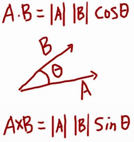
Step 4: Dot and Cross Product between Vectors
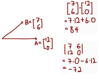
Let's revisit the vector operations: dot product and cross product. This is not a Math class, and we have covered these in more detail before, but still, it's good to refresh our memory on the workings so I've included the image above. The diagram shows "B dot A" operation (top right corner) and "B cross A" operation (bottom right corner).
More important are the equations of these operations. Take a look at the image below. |A| and |B| refer to the scalar magnitude of each vector - the length of the arrow. Note that the dot product relates to the cosine of the angle between the vectors, and the cross product relates to the sine of the angle between the vectors.
Step 5: Sine and Cosine
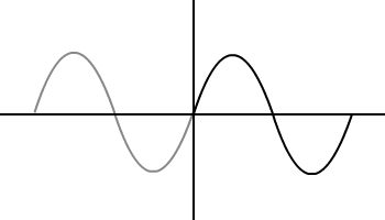
Drilling further into the topic, Trigonometry comes to play: the sine and cosine. Im sure these graphs rekindle fond memories (or agonies). Do click on the buttons on Flash presentation below to view those graphs with different units (degrees or radians).
Note that these wave forms are continuous and repetitive. For example, you can cut and paste the sine wave into the negative range to get something like below.
Step 6: Summary of Values
| Degree | Sine of degree | Cosine of degree |
| -180 | 0 | -1 |
| -90 | -1 | 0 |
| 0 | 0 | 1 |
| 90 | 1 | 0 |
| 180 | 0 | -1 |
The table above shows the cosine and sine values corresponding to specific degrees. You'll notice the positive sine graph covers 0° to 180° range and positive cosine graph covers -90° to 90°. We shall relate these values to the dot product and cross product later.
Step 7: Geometric Interpretation of Dot Product
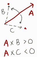
So how can all these be useful? To cut to the chase, the dot product is a measure of how parallel the vectors are whereas cross product is a measure of how orthogonal the vectors are.
Lets deal with the dot product first. Recall the formula for the dot product, as mentioned in Step 4. We can determine the whether result is positive or negative just by looking at the cosine of the angle sandwiched between the two vectors. Why? Because the magnitude of a vector is always positive. The only parameter left to dictate the sign of the result is the cosine of the angle.
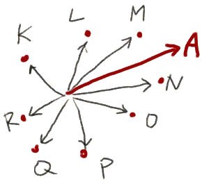
Again, recall that positive cosine graph covers -90° - 90°, as in Step 6. Therefore, the dot product of A with any of the vecotrs L, M, N, O above will produce a positive value, because the angle wedged between A and any of those vectors is within -90° and 90°! (To be precise, the positive range is more like -89° - 89° because both -90° and 90° produces cosine values of 0, which brings us to the next point.) The dot product between A and P (given P is perpendicular to A) will produce 0. The rest I think you can already guess: the dot product of A with K, R, or Q will produce a negative value.
By using the dot product, we can split the area on our stage into two regions. The dot product of the vector below with any point that lies inside of the "x"-marked region will produce a positive value, whereas the dot product with those in the "o"-marked region will produce negative values.
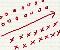
Step 8: Geometric Interpretation of Cross Product
Let's move on to the cross product. Remember that the cross product relates to the sine of angle sandwiched between the two vectors. The positive sine graph covers a range of 0° to 180°; the negative range covers 0° to -180°. The image below summarises these points.
So, looking again at the diagram from Step 7, the cross product between A and K, L, or M will produce positive values, while the cross product between A and N, O, P, or Q will produce negative values. The cross product between A and R will produce 0, as sine of 180° is 0.
To clarify further, the cross product of vector between any point that lies in the "o"-marked region below will be positive, whereas those in "x"-marked region will be negative.
One point to take note of is that, unlike the dot product, the cross product is sequence sensitive. This means results of AxB and BxA will be different in terms of direction. So as we write our program, we need to be precise when choosing which vector to be compared against.
(Note: These concepts explained apply to 2D Cartesian space.)
Step 9: Demo Application
To reinforce your understanding, I've placed here a little application to let you play with. Click on the blue ball at the top of stage and drag it around. As you move, the text box value will update depending on which operation you have chosen (dot or cross product between the static arrow with the one you control).
You may observe one oddity with the cross product's inverted direction. The region on top is negative and the bottom is positive, in contrast with our explanation in previous step. Well, this is due to the y-axis being inverted in Flash coordinate space compared to Cartesian coordinate space; it points down, whereas traditionally mathematicians take it as pointing upwards.
Step 10: Defining Regions
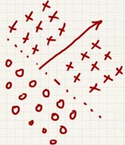
Now that you have understood the concept of regions, let's do a little practice. We shall divide our space into four quadrants: A1, A2, B1, B2.
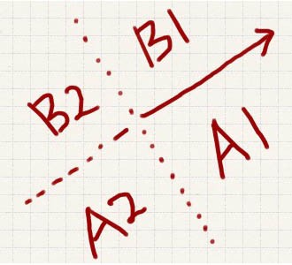
I've tabulated the results to check for below. "Vector" here refers to the arrow in the image above. "Point" refers to any coordinate in the specified region. The vector divides the stage into four main areas, where the dividers (dotted lines) extend to infinity.
| Region | Vector on diagram cross product with point | Vector on diagram dot product with point |
| A1 | (+), because of Flash coordinate space | (+) |
| A2 | (+) | (-) |
| B1 | (-), because of Flash coordinate space | (+) |
| B2 | (-) | (-) |
Step 11: Regions Divided
Here's the Flash presentation showcasing the ideas as explained in step 10. Right click on stage to pop the context menu and select the region you would like to see highlighted.
Step 12: Implementation
Here's the ActionScript implementation of the concept explained in Step 10. Feel free to view the whole piece of code in the source download, as AppLine.as.
//highlighting color according to user selection
private function color():void
{
	//each ball on stage is checked against conditions for selected case
	for each (var item:Ball in sp)
	{
		var vec1:Vector2D = new Vector2D(item.x - stage.stageWidth * 0.5, item.y - stage.stageHeight * 0.5);

		if (select == 0) {
			if (vec.vectorProduct(vec1) > 0) item.col = 0xFF9933;
			else item.col = 0x334455;
		}
		else if (select == 1){
			if (vec.dotProduct(vec1) > 0) item.col = 0xFF9933;
			else item.col = 0x334455;
		}
		else if (select == 2){
			if (vec.vectorProduct(vec1) > 0 && vec.dotProduct(vec1) > 0) item.col = 0xFF9933;
			else item.col = 0x334455;
		}
		else if (select == 3){
			if (vec.vectorProduct(vec1) > 0 &&vec.dotProduct(vec1) <0) item.col = 0xFF9933;
			else item.col = 0x334455;
		}
		else if (select == 4){
			if (vec.vectorProduct(vec1) < 0 &&vec.dotProduct(vec1) > 0) item.col = 0xFF9933;
			else item.col = 0x334455;
		}
		else if (select == 5){
			if (vec.vectorProduct(vec1) < 0 &&vec.dotProduct(vec1) < 0) item.col = 0xFF9933;
			else item.col = 0x334455;
		}
		item.draw();
	}
}
//swapping case according to user selction
private function swap(e:ContextMenuEvent):void
{
	if (e.target.caption == "VectorProduct")	select = 0;
	else if (e.target.caption == "DotProduct")	select = 1;
	else if (e.target.caption == "RegionA1")	select = 2;
	else if (e.target.caption == "RegionA2")	select = 3;
	else if (e.target.caption == "RegionB1")	select = 4;
	else if (e.target.caption == "RegionB2")	select = 5;
}
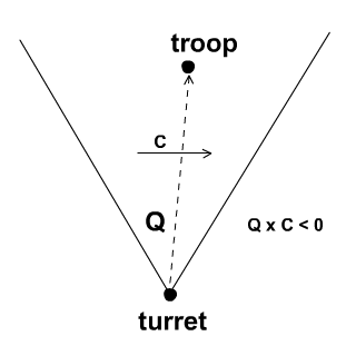
Step 13: Shielded Visibility
Having understood the geometrical interpretations of dot product and cross product, we shall apply it to our scenario. The Flash presentation above shows variations of the same scenario and summarises the conditions applied to a trooper shielded by a wall yet inside the turret's FOV. You can scroll through the frames using the arrow buttons.
The following explanations are based upon the 2D Flash coordinate space. In Frame 1, a wall is placed between the turret and the trooper. Let A and B be the vectors from the turret to the tail and the head of the wall's vector, respectively. Let C be the vector of the wall, and D be the vector from the tail of the wall to the trooper. Finally, let Q be the vector from the turret to the trooper.
I have tabulated the resulting conditions below.
| Location | Cross Product |
| Troop is in front of wall | C x D > 0 |
| Troop is behind wall | C x D |
This is not the only condition applicable, because we also need to restrict the trooper to within the dotted lines on both sides. Check out frames 2-4 to see the next set of conditions.
| Location | Cross Product |
| Troop is within the sides of the wall. | Q x A 0 |
| Troop is to the left of the wall | Q x A > 0, Q x B > 0 |
| Troop is to the right of the wall | Q x A |
I think my fellow readers can now choose the appropriate conditions to determine whether the trooper is hidden from view or not. Bear in mind that this set of conditions are evaluated after we found troop to be within turret's FOV (refer to step 3).
Step 14: Actionscript Implementation
Here's the ActionScript implementation of the concepts explained in Step 13. The image above shows the initial vector of the wall, C. Click and drag the red button below and move it around to see the area shielded. You may view the full source code in HiddenSector.as.
Okay, I hope you have experimented with the red ball, and if you are observant enough you might have noticed an error. Note there is no area shielded as the red button moves to the left of the other end of the wall, thus inverting the wall vector to point to left instead of right. The solution is in the next step.
However, before that let's look at an important ActionScript snippet here in HiddenSector.as:
private function highlight():void {
	var lineOfSight:Vector2D = new Vector2D(0, -50)
	var sector:Number = Math2.radianOf(30);

	for each (var item:Ball in sp) {
		var turret_sp:Vector2D = new Vector2D(item.x - turret.x, item.y - turret.y); //Q

		if (Math.abs(lineOfSight.angleBetween(turret_sp)) < sector) {

			var wall:Vector2D = new Vector2D(wall2.x - wall1.x, wall2.y - wall1.y); //C
			var turret_wall1:Vector2D = new Vector2D(wall1.x - turret.x, wall1.y - turret.y); //A
			var turret_wall2:Vector2D = new Vector2D(wall2.x - turret.x, wall2.y - turret.y); //B
			var wall_sp:Vector2D = new Vector2D (item.x - wall1.x, item.y - wall1.y); //D

			if ( wall.vectorProduct (wall_sp) < 0 // C x D
			&& turret_sp.vectorProduct(turret_wall1) < 0 // Q x A
			&& turret_sp.vectorProduct(turret_wall2) > 0 // Q x B
			) { item.col = 0xcccccc }
			else { item.col = 0; }
			item.draw();
		}
	}
}
Step 15: Direction of Wall
To solve this issue, we need to know whether the wall vector is pointing to the left or the right. Let's say we have a reference vector, R, that's always pointing to the right.
| Direction of vector | Dot Product |
| Wall is pointing to right (same side as R) | w . R > 0 |
| Wall is pointing to left (opposite side of R) | w . R |
Of course, there are other ways around this problem but I figure it's an opportunity to utilise concepts expressed in this tutorial, so there you go.
Step 16: Actionscript Tweaks
Below is a Flash presentation which implements the correction explained in Step 15. After you have played with it, scroll down to check the ActionScript tweaks.
The changes from the previous implementation are highlighted. Also, the sets of condition are redefined according to the wall direction:
private function highlight():void {
	var lineOfSight:Vector2D = new Vector2D(0, -50);
	var sector:Number = Math2.radianOf(30);
	var pointToRight:Vector2D = new Vector2D(10, 0); //added in second version

	for each (var item:Ball in sp) {
		var turret_sp:Vector2D = new Vector2D(item.x - turret.x, item.y - turret.y); //Q

		if (Math.abs(lineOfSight.angleBetween(turret_sp)) < sector) {

			var wall:Vector2D = new Vector2D(wall2.x - wall1.x, wall2.y - wall1.y); //C
			var turret_wall1:Vector2D = new Vector2D(wall1.x - turret.x, wall1.y - turret.y); //A
			var turret_wall2:Vector2D = new Vector2D(wall2.x - turret.x, wall2.y - turret.y); //B
			var wall_sp:Vector2D = new Vector2D (item.x - wall1.x, item.y - wall1.y); //D

			var sides: Boolean; //switches according to wall direction
			if (pointToRight.dotProduct(wall) > 0) {
				sides = wall.vectorProduct (wall_sp) < 0 // C x D
				&& turret_sp.vectorProduct(turret_wall1) < 0 // Q x A
				&& turret_sp.vectorProduct(turret_wall2) > 0 // Q x B
			}
			else {
				sides = wall.vectorProduct (wall_sp) > 0 // C x D
				&& turret_sp.vectorProduct(turret_wall1) > 0 // Q x A
				&& turret_sp.vectorProduct(turret_wall2) < 0 // Q x B
			}

			if (sides) { item.col = 0xcccccc }
			else { item.col = 0; }
			item.draw();
		}
	}
}
Check out the full source in HiddenSector2.as.
Step 17: Set Up the Wall
Now we shall patch our work onto Scene1.as from the previous tutorial. First, we shall set up our wall.
We initiate the variables,
public class Scene1_2 extends Sprite
{
	private var river:Sprite;
	private var wall_origin:Vector2D, wall:Vector2D; //added in second tutorial

	private var troops:Vector.<Ball>;
	private var troopVelo:Vector.<Vector2D>;
...then draw the wall for the first time,
public function Scene1_2() {
	makeTroops();
	makeRiver();
	makeWall(); //added in 2nd tutorial
	makeTurret();
	turret.addEventListener(MouseEvent.MOUSE_DOWN, start);
	function start ():void {
		stage.addEventListener(Event.ENTER_FRAME, move);
	}
}
private function makeWall():void {
	wall_origin = new Vector2D(200, 260); wall = new Vector2D(80, -40);
	graphics.lineStyle(2, 0);
	graphics.moveTo(wall_origin.x, wall_origin.y);
	graphics.lineTo(wall_origin.x + wall.x , wall_origin.y+wall.y);
}
...and redraw on each frame, because the graphics.clear() call is somewhere in behaviourTurret():
//added in 2nd tutorial
private function move(e:Event):void {
	behaviourTroops();
	behaviourTurret();
	redrawWall();
}
//added in second tutorial
private function redrawWall():void {
	graphics.lineStyle(2, 0);
	graphics.moveTo(wall_origin.x, wall_origin.y);
	graphics.lineTo(wall_origin.x + wall.x , wall_origin.y+wall.y);
}
Step 18: Interaction with Wall
Troops will interact with the wall as well. As they collide with the wall, they will slide along the wall. I will not try to go into details of this as it has been documented extensively in Collision Reaction Between a Circle and a Line Segment. I encourage readers to check that out for further explanation.
The following snippet lives in the function behaviourTroops().
//Version 2
//if wading through river, slow down
//if collide with wall, slide through
//else normal speed
var collideWithRiver:Boolean = river.hitTestObject(troops[i])

var wall_norm:Vector2D = wall.rotate(Math2.radianOf( -90));
var wall12Troop:Vector2D = new Vector2D(troops[i].x - wall_origin.x, troops[i].y - wall_origin.y);
var collideWithWall:Boolean = troops[i].rad > Math.abs(wall12Troop.projectionOn(wall_norm))
&& wall12Troop.getMagnitude() < wall.getMagnitude()
&& wall12Troop.dotProduct(wall) > 0;

if (collideWithRiver) troops[i].y += troopVelo[i].y*0.3;
else if (collideWithWall) {
	//reposition troop
	var projOnNorm:Vector2D = wall_norm.normalise(); projOnNorm.scale(troops[i].rad -1);
	var projOnWall:Vector2D = wall.normalise();
	projOnWall.scale(wall12Troop.projectionOn(wall));
	var reposition:Vector2D = projOnNorm.add(projOnWall);
	troops[i].x = wall_origin.x + reposition.x; troops[i].y = wall_origin.y + reposition.y;

	//slide through the wall
	var adjustment:Number = Math.abs(troopVelo[i].projectionOn(wall_norm));
	var slideVelo:Vector2D = wall_norm.normalise(); slideVelo.scale(adjustment);
	slideVelo = slideVelo.add(troopVelo[i])
	troops[i].x += slideVelo.x; troops[i].y += slideVelo.y;
}
else troops[i].y += troopVelo[i].y
Step 19: Checking Troopers' "Hidden-ness"
Finally, we come to the meat of this tutorial: setting up the condition and checking whether troopers are behind the wall and therefore shielded from turret visibility. I have highlighted the important patch codes:
//check if enemy is within sight
//1. Within sector of view
//2. Within range of view
//3. Closer than current closest enemy
var c1:Boolean = Math.abs(lineOfSight.angleBetween(turret2Item)) < Math2.radianOf(sectorOfSight) ;
var c2:Boolean = turret2Item.getMagnitude() < lineOfSight.getMagnitude();
var c3:Boolean = turret2Item.getMagnitude() < closestDistance;

//Checking whether troop is shielded by wall
var withinLeft:Boolean = turret2Item.vectorProduct(turret2wall1) < 0
var withinRight:Boolean = turret2Item.vectorProduct(turret2wall2) > 0
var behindWall:Boolean = wall.vectorProduct(wall12troop) < 0;
var shielded:Boolean = withinLeft && withinRight && behindWall

//if all conditions fulfilled, update closestEnemy
if (c1 && c2&& c3 && !shielded){
	closestDistance = turret2Item.getMagnitude();
	closestEnemy = item;
}
Check out the full code in Scene1_2.as.
Step 20: Lauch the Application
Finally, we can sit back and check out the patch in action. Hit Ctrl + Enter to see the results of your work. I have included a copy of the working Flash presentation below. Click on the turret at the bottom of the stage to start the simulation.

Comments