So far we’ve looked at data structures that organize data in a linear fashion. Linked lists contain data from a single starting node to a single terminating node. Arrays hold data in contiguous, one-dimensional blocks.
Overview
In this section, we will see how adding one more dimension will allow us to introduce a new data structure: the tree. Specifically, we will be looking at a type of tree known as a binary search tree. Binary search trees take the general tree structure and apply a set of simple rules that define the tree's structure.
Before we learn about those rules, let’s learn what a tree is.
Tree Overview
A tree is a data structure where each node has zero or more children. For example, we might have a tree like this:

In this tree, we can see the organizational structure of a business. The blocks represent people or divisions within the company, and the lines represent reporting relationships. A tree is a very efficient, logical way to present and store this information.
The tree shown in the previous figure is a general tree. It represents parent/child relationships, but there are no rules for the structure. The CEO has one direct report but could just as easily have none or twenty. In the figure, Sales is shown to the left of Marketing, but that ordering has no meaning. In fact, the only observable constraint is that each node has at most one parent (and the top-most node, the Board of Directors, has no parent).
Binary Search Tree Overview
A binary search tree uses the same basic structure as the general tree shown in the last figure but with the addition of a few rules. These rules are:
- Each node can have zero, one, or two children.
- Any value less than the node’s value goes to the left child (or a child of the left child).
- Any value greater than, or equal to, the node’s value goes to the right child (or a child thereof).
Let’s look at a tree that is built using these rules:
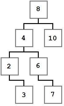
Notice how the constraints we specified are enforced in the diagram. Every value to the left of the root node (eight) has a value less than eight, and every value to the right is greater than or equal to the root node. This rule applies recursively at every node along the way.
With this tree in mind, let’s think about the steps that went into building it. When the process started, the tree was empty and then a value, eight, was added. Because it was the first value added, it was put into the root (ultimate parent) position.
We don’t know the exact order that the rest of the nodes were added, but I’ll present one possible path. Values will be added using a method named Add that accepts the value.
BinaryTree tree = new BinaryTree();
tree.Add(8);
tree.Add(4);
tree.Add(2);
tree.Add(3);
tree.Add(10);
tree.Add(6);
tree.Add(7);
Let’s walk through the first few items.
Eight was added first and became the root. Next, four was added. Since four is less than eight, it needs to go to the left of eight as per rule number two. Since eight has no child on its left, four becomes the immediate left child of eight.
Two is added next. two is less than eight, so it goes to the left. There is already a node to the left of eight, so the comparison logic is performed again. two is less than four, and four has no left child, so two becomes the left child of four.
Three is added next and goes to the left of eight and four. When compared to the two node, it is larger, so three is added to the right of two as per rule number three.
This cycle of comparing values at each node and then checking each child over and over until the proper slot is found is repeated for each value until the final tree structure is created.
The Node Class
The BinaryTreeNode represents a single node in the tree. It contains references to the left and right children (null if there are none), the node’s value, and the IComparable.CompareTo method which allows comparing the node values to determine if the value should go to the left or right of the current node. This is the entire BinaryTreeNode class—as you can see, it is very simple.
class BinaryTreeNode : IComparable
	where TNode : IComparable
{
	public BinaryTreeNode(TNode value)
	{
		Value = value;
	}

	public BinaryTreeNode Left { get; set; }
	public BinaryTreeNode Right { get; set; }
	public TNode Value { get; private set; }

	///
	/// Compares the current node to the provided value.
	///
	/// The node value to compare to
	/// 1 if the instance value is greater than
	/// the provided value, -1 if less, or 0 if equal.
	public int CompareTo(TNode other)
	{
		return Value.CompareTo(other);
	}
}
The Binary Search Tree Class
The BinaryTree class provides the basic methods you need to manipulate the tree: Add, Remove, a Contains method to determine if an item exists in the tree, several traversal and enumeration methods (these are methods that allow us to enumerate the nodes in the tree in various well-defined orders), and the normal Count and Clear methods.
To initialize the tree, there is a BinaryTreeNode reference that represents the head (root) node of the tree, and there is an integer that keeps track of how many items are in the tree.
public class BinaryTree : IEnumerable
	where T : IComparable
{
	private  BinaryTreeNode _head;
	private int _count;

	public void Add(T value)
	{
		throw new NotImplementedException();
	}

	public bool Contains(T value)
	{
		throw new NotImplementedException();
	}

	public bool Remove(T value)
	{
		throw new NotImplementedException();
	}

	public void PreOrderTraversal(Action action)
	{
		throw new NotImplementedException();
	}

	public void PostOrderTraversal(Action action)
	{
		throw new NotImplementedException();
	}

	public void InOrderTraversal(Action action)
	{
		throw new NotImplementedException();
	}

	public IEnumerator GetEnumerator()
	{
		throw new NotImplementedException();
	}

	System.Collections.IEnumerator System.Collections.IEnumerable.GetEnumerator()
	{
		throw new NotImplementedException();
	}

	public void Clear()
	{
		throw new NotImplementedException();
	}

	public int Count
	{
		get;
	}
}
Add
| Behavior | Adds the provided value to the correct location within the tree. |
| Performance | O(log n) on average; O(n) in the worst case. |
Adding a node to the tree isn’t terribly complex and is made even easier when the problem is simplified into a recursive algorithm. There are two cases that need to be considered:
- The tree is empty.
- The tree is not empty.
In the first case, we simply allocate the new node and add it to the tree. In the second case, we compare the value to the node’s value. If the value we are trying to add is less than the node’s value, the algorithm is repeated for the node’s left child. Otherwise, it is repeated for the node’s right child.
public void Add(T value)
{
	// Case 1: The tree is empty. Allocate the head.
	if (_head == null)
	{
		_head = new BinaryTreeNode(value);
	}
	// Case 2: The tree is not empty, so recursively
	// find the right location to insert the node.
	else
	{
		AddTo(_head, value);
	}

	_count++;
}

// Recursive add algorithm.
private void AddTo(BinaryTreeNode node, T value)
{
	// Case 1: Value is less than the current node value
	if (value.CompareTo(node.Value) < 0)
	{
		// If there is no left child, make this the new left,
		if (node.Left == null)
		{
			node.Left = new BinaryTreeNode(value);
		}
		else
		{
			// else add it to the left node.
			AddTo(node.Left, value);
		}
	}
	// Case 2: Value is equal to or greater than the current value.
	else
	{
		// If there is no right, add it to the right,
		if (node.Right == null)
		{
			node.Right = new BinaryTreeNode(value);
		}
		else
		{
			// else add it to the right node.
			AddTo(node.Right, value);
		}
	}
}
Remove
| Behavior | Removes the first nore found with the indicated value. |
| Performance | O(log n) on average; O(n) in the worst case. |
Removing a value from the tree is a conceptually simple operation that becomes surprisingly complex in practice.
At a high level, the operation is simple:
- Find the node to remove
- Remove it.
The first step is simple, and as we’ll see, is accomplished using the same mechanism that the Contains method uses. Once the node to be removed is identified, however, the operation can take one of three paths dictated by the state of the tree around the node to be removed. The three states are described in the following three cases.
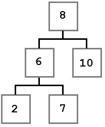
Case One: The node to be removed has no right child.
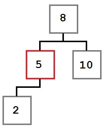
In this case, the removal operation can simply move the left child, if there is one, into the place of the removed node. The resulting tree would look like this:
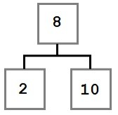
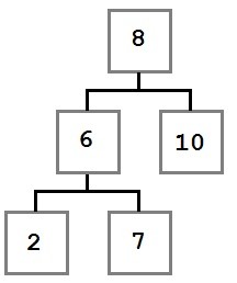
Case Two: The node to be removed has a right child which, in turn, has no left child.
In this case, we want to move the removed node’s right child (six) into the place of the removed node. The resulting tree will look like this:
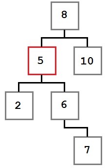
Case Three: The node to be removed has a right child which, in turn, has a left child.
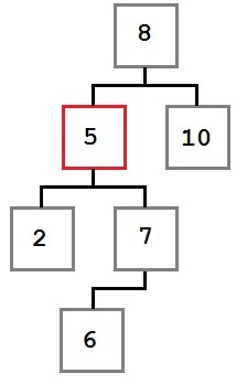
In this case, the left-most child of the removed node’s right child must be placed into the removed node’s slot.
Let’s take a minute to think about why this is true. There are two facts that we know about the sub-tree starting with the node being removed (for example, the sub-tree whose root is the node with the value five).
- Every value to the right of the node is greater than or equal to five.
- The smallest value in the right sub-tree is the left-most node.
We need to place a value into the removed node’s slot which is smaller than, or equal to, every node to its right. To do that, we need to get the smallest value on the right side. Therefore we need the right child’s left-most node.
After the node removal, the tree will look like this:
Now that we understand the three remove scenarios, let’s look at the code to make it happen.
One thing to note: The FindWithParent method (see the Contains section) returns the node to remove as well as the parent of the node being removed. This is done because when the node is removed, we need to update the parent’s Left or Right property to point to the new node.
We could avoid doing this if all nodes kept a reference to their parent, but that would introduce per-node memory overhead and bookkeeping costs that are only needed in this one case.
public bool Remove(T value)
{
	BinaryTreeNode current, parent;

	// Find the node to remove.
	current = FindWithParent(value, out parent);

	if (current == null)
	{
		return false;
	}

	_count--;

	// Case 1: If current has no right child, current's left replaces current.
	if (current.Right == null)
	{
		if (parent == null)
		{
			_head = current.Left;
		}
		else
		{
			int result = parent.CompareTo(current.Value);
			if (result > 0)
			{
				// If parent value is greater than current value,
				// make the current left child a left child of parent.
				parent.Left = current.Left;
			}
			else if (result < 0)
			{
				// If parent value is less than current value,
				// make the current left child a right child of parent.
				parent.Right = current.Left;
			}
		}
	}
	// Case 2: If current's right child has no left child, current's right child
	//         replaces current.
	else if (current.Right.Left == null)
	{
		current.Right.Left = current.Left;

		if (parent == null)
		{
			_head = current.Right;
		}
		else
		{
			int result = parent.CompareTo(current.Value);
			if (result > 0)
			{
				// If parent value is greater than current value,
				// make the current right child a left child of parent.
				parent.Left = current.Right;
			}
			else if (result < 0)
			{
				// If parent value is less than current value,
				// make the current right child a right child of parent.
				parent.Right = current.Right;
			}
		}
	}
	// Case 3: If current's right child has a left child, replace current with current's
	//         right child's left-most child.
	else
	{
		// Find the right's left-most child.
		BinaryTreeNode leftmost = current.Right.Left;
		BinaryTreeNode leftmostParent = current.Right;

		while (leftmost.Left != null)
		{
			leftmostParent = leftmost;
			leftmost = leftmost.Left;
		}

		// The parent's left subtree becomes the leftmost's right subtree.
		leftmostParent.Left = leftmost.Right;

		// Assign leftmost's left and right to current's left and right children.
		leftmost.Left = current.Left;
		leftmost.Right = current.Right;

		if (parent == null)
		{
			_head = leftmost;
		}
		else
		{
			int result = parent.CompareTo(current.Value);
			if (result > 0)
			{
				// If parent value is greater than current value,
				// make leftmost the parent's left child.
				parent.Left = leftmost;
			}
			else if (result < 0)
			{
				// If parent value is less than current value,
				// make leftmost the parent's right child.
				parent.Right = leftmost;
			}
		}
	}

	return true;
}
Contains
| Behavior | Returns true if the tree contains the provided value. Otherwise it returns false. |
| Performance | O(log n) on average; O(n) in the worst case. |
Contains defers to FindWithParent, which performs a simple tree-walking algorithm that performs the following steps, starting at the head node:
- If the current node is null, return null.
- If the current node value equals the sought value, return the current node.
- If the sought value is less than the current value, set the current node to left child and go to step number one.
- Set current node to right child and go to step number one.
Since Contains returns a Boolean, the returned value is determined by whether FindWithParent returns a non-null BinaryTreeNode (true) or a null one (false).
The FindWithParent method is used by the Remove method as well. The out parameter, parent, is not used by Contains.
public bool Contains(T value)
{
	// Defer to the node search helper function.
	BinaryTreeNode parent;
	return FindWithParent(value, out parent) != null;
}

///
/// Finds and returns the first node containing the specified value. If the value
/// is not found, it returns null. Also returns the parent of the found node (or null)
/// which is used in Remove.
///
private BinaryTreeNode FindWithParent(T value, out BinaryTreeNode parent)
{
	// Now, try to find data in the tree.
	BinaryTreeNode current = _head;
	parent = null;

	// While we don't have a match...
	while (current != null)
	{
		int result = current.CompareTo(value);

		if (result > 0)
		{
			// If the value is less than current, go left.
			parent = current;
			current = current.Left;
		}
		else if (result < 0)
		{
			// If the value is more than current, go right.
			parent = current;
			current = current.Right;
		}
		else
		{
			// We have a match!
			break;
		}
	}

	return current;
}
Count
| Behavior | Returns the number of values in the tree (0 if empty). |
| Performance | O(1) |
The count field is incremented by the Add method and decremented by the Remove method.
public int Count
{
	get
	{
		return _count;
	}
}
Clear
| Behavior | Removes all the nodes from the tree. |
| Performance | O(1) |
public void Clear()
{
	_head = null;
	_count = 0;
}
Traversals
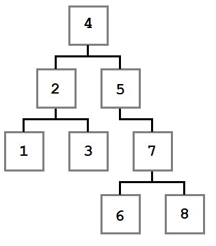
Tree traversals are algorithms that allow processing each value in the tree in a well-defined order. For each of the algorithms discussed, the following tree will be used as the sample input.
The examples that follow all accept an Action<T> parameter. This parameter defines the action that will be applied to each node as it is processed by the traversal.
The Order section for each traversal will indicate the order in which the following tree would traverse.
Preorder
| Behavior | Performs the provided action on each value in preorder (see the description that follows). |
| Performance | O(n) |
| Order | 4, 2, 1, 3, 5, 7, 6, 8 |
The preorder traversal processes the current node before moving to the left and then right children. Starting at the root node, four, the action is executed with the value four. Then the left node and all of its children are processed, followed by the right node and all of its children.
A common usage of the preorder traversal would be to create a copy of the tree that contained not just the same node values, but also the same hierarchy.
public void PreOrderTraversal(Action action)
{
	PreOrderTraversal(action, _head);
}

private void PreOrderTraversal(Action action, BinaryTreeNode node)
{
	if (node != null)
	{
		action(node.Value);
		PreOrderTraversal(action, node.Left);
		PreOrderTraversal(action, node.Right);
	}
}
Postorder
| Behavior | Performs the provided action on each value in postorder (see the description that follows). |
| Performance | O(n) |
| Order | 1, 3, 2, 6, 8, 7, 5, 4 |
The postorder traversal visits the left and right child of the node recursively, and then performs the action on the current node after the children are complete.
Postorder traversals are often used to delete an entire tree, such as in programming languages where each node must be freed, or to delete subtrees. This is the case because the root node is processed (deleted) last and its children are processed in a way that will minimize the amount of work the Remove algorithm needs to perform.
public void PostOrderTraversal(Action action)
{
	PostOrderTraversal(action, _head);
}

private void PostOrderTraversal(Action action, BinaryTreeNode node)
{
	if (node != null)
	{
		PostOrderTraversal(action, node.Left);
		PostOrderTraversal(action, node.Right);
		action(node.Value);
	}
}
Inorder
| Behavior | Performs the provided action on each value in inorder (see the description that follows). |
| Performance | O(n) |
| Order | 1, 2, 3, 4, 5, 6, 7, 8 |
Inorder traversal processes the nodes in the sort order—in the previous example, the nodes would be sorted in numerical order from smallest to largest. It does this by finding the smallest (left-most) node and then processing it before processing the larger (right) nodes.
Inorder traversals are used anytime the nodes must be processed in sort-order.
The example that follows shows two different methods of performing an inorder traversal. The first implements a recursive approach that performs a callback for each traversed node. The second removes the recursion through the use of the Stack data structure and returns an IEnumerator to allow direct enumeration.
Public void InOrderTraversal(Action action)
{
	InOrderTraversal(action, _head);
}

private void InOrderTraversal(Action action, BinaryTreeNode node)
{
	if (node != null)
	{
		InOrderTraversal(action, node.Left);

		action(node.Value);

		InOrderTraversal(action, node.Right);
	}
}

public IEnumerator InOrderTraversal()
{
	// This is a non-recursive algorithm using a stack to demonstrate removing
	// recursion.
	if (_head != null)
	{
		// Store the nodes we've skipped in this stack (avoids recursion).
		Stack> stack = new Stack>();

		BinaryTreeNode current = _head;

		// When removing recursion, we need to keep track of whether
		// we should be going to the left node or the right nodes next.
		bool goLeftNext = true;

		// Start by pushing Head onto the stack.
		stack.Push(current);

		while (stack.Count > 0)
		{
			// If we're heading left...
			if (goLeftNext)
			{
				// Push everything but the left-most node to the stack.
				// We'll yield the left-most after this block.
				while (current.Left != null)
				{
					stack.Push(current);
					current = current.Left;
				}
			}

			// Inorder is left->yield->right.
			yield return current.Value;

			// If we can go right, do so.
			if (current.Right != null)
			{
				current = current.Right;

				// Once we've gone right once, we need to start
				// going left again.
				goLeftNext = true;
			}
			else
			{
				// If we can't go right, then we need to pop off the parent node
				// so we can process it and then go to its right node.
				current = stack.Pop();
				goLeftNext = false;
			}
		}
	}
}
GetEnumerator
| Behavior | Returns an enumerator that enumerates using the InOrder traversal algorithm. |
| Performance | O(1) to return the enumerator. Enumerating all the items is O(n). |
public IEnumerator GetEnumerator()
{
	return InOrderTraversal();
}

System.Collections.IEnumerator System.Collections.IEnumerable.GetEnumerator()
{
	return GetEnumerator();
}

Comments