In this section, we are going to look at five algorithms used to sort data in an array. We will start with a naïve algorithm, bubble sort, and end with the most common general purpose sorting algorithm, quick sort.
With each algorithm I will explain how the sorting is done and also provide information on the best, average, and worst case complexity for both performance and memory usage.
Swap
To keep the sorting algorithm code a little easier to read, a common Swap method will be used by any sorting algorithm that needs to swap values in an array by index.
void Swap(T[] items, int left, int right)
{
	if (left != right)
	{
		T temp = items[left];
		items[left] = items[right];
		items[right] = temp;
	}
}
Bubble Sort
| Behavior | Sorts the input array using the bubble sort algorithm. | ||
| Complexity | Best Case | Average Case | Worst Case |
| Time | O(n) | O(n2) | O(n2) |
| Space | O(1) | O(1) | O(1) |
Bubble sort is a naïve sorting algorithm that operates by making multiple passes through the array, each time moving the largest unsorted value to the right (end) of the array.
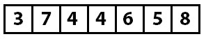
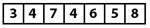
Consider the following unsorted array of integers:
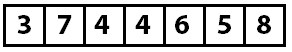
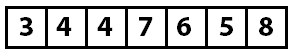
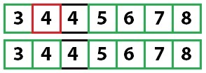
On the first pass through the array, the values three and seven are compared. Since seven is larger than three, no swap is performed. Next, seven and four are compared. Seven is greater than four so the values are swapped, thus moving the seven, one step closer to the end of the array. The array now looks like this:
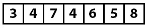
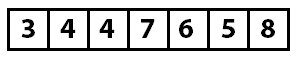
This process is repeated, and the seven eventually ends up being compared to the eight, which is greater, so no swapping can be performed, and the pass ends at the end of the array. At the end of pass one, the array looks like this:
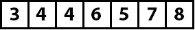
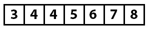
Because at least one swap was performed, another pass will be performed. After the second pass, the six has moved into position.
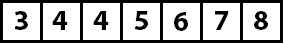
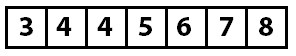
Again, because at least one swap was performed, another pass is performed.
The next pass, however, finds that no swaps were necessary because all of the items are in sort-order. Since no swaps were performed, the array is known to be sorted and the sorting algorithm is complete.
public void Sort(T[] items)
{
	bool swapped;

	do
	{
		swapped = false;
		for (int i = 1; i < items.Length; i++)
		{
			if (items[i - 1].CompareTo(items[i]) > 0)
			{
				Swap(items, i - 1, i);
				swapped = true;
			}
		}
	} while (swapped != false);
}
Insertion Sort
| Behavior | Sorts the input array using the insertion sort algorithm. | ||
| Complexity | Best Case | Average Case | Worst Case |
| Time | O(n) | O(n2) | O(n2) |
| Space | O(1) | O(1) | O(1) |
Insertion sort works by making a single pass through the array and inserting the current value into the already sorted (beginning) portion of the array. After each index is processed, it is known that everything encountered so far is sorted and everything that follows is unknown.
Wait, what?
The important concept is that insertion sort works by sorting items as they are encountered. Since it processes the array from left to right, we know that everything to the left of the current index is sorted. This graphic demonstrates how the array becomes sorted as each index is encountered:
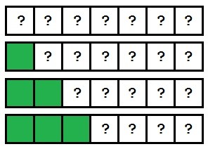
As the processing continues, the array becomes more and more sorted until it is completely sorted.
Let’s look at a concrete example. The following is an unsorted array that will be sorted using insertion sort.
When the sorting process begins, the sorting algorithm starts at index zero with the value three. Since there are no values that precede this, the array up to and including index zero is known to be sorted.
The algorithm then moves on to the value seven. Since seven is greater than everything in the known sorted range (which currently only includes three), the values up to and including seven are known to be in sort-order.
At this point the array indexes 0-1 are known to be sorted, and 2-n are in an unknown state.
The value at index two (four) is checked next. Since four is less than seven, it is known that four needs to be moved into its proper place in the sorted array area. The question now is to which index in the sorted array should the value be inserted. The method to do this is the FindInsertionIndex shown in the code sample. This method compares the value to be inserted (four) against the values in the sorted range, starting at index zero, until it finds the point at which the value should be inserted.
This method determines that index one (between three and seven) is the appropriate insertion point. The insertion algorithm (the Insert method) then performs the insertion by removing the value to be inserted from the array and shifting all the values from the insertion point to the removed item to the right. The array now looks like this:
The array from index zero to two is now known to be sorted, and everything from index three to the end is unknown. The process now starts again at index three, which has the value four. As the algorithm continues, the following insertions occur until the array is sorted.
When there are no further insertions to be performed, or when the sorted portion of the array is the entire array, the algorithm is finished.
public void Sort(T[] items)
{
	int sortedRangeEndIndex = 1;

	while (sortedRangeEndIndex < items.Length)
	{
		if (items[sortedRangeEndIndex].CompareTo(items[sortedRangeEndIndex - 1]) < 0)
		{
			int insertIndex = FindInsertionIndex(items, items[sortedRangeEndIndex]);
			Insert(items, insertIndex, sortedRangeEndIndex);
		}

		sortedRangeEndIndex++;
	}
}

private int FindInsertionIndex(T[] items, T valueToInsert)
{
	for (int index = 0; index < items.Length; index++)
	{
		if (items[index].CompareTo(valueToInsert) > 0)
		{
			return index;
		}
	}

	throw new InvalidOperationException("The insertion index was not found");
}

private void Insert(T[] itemArray, int indexInsertingAt, int indexInsertingFrom)
{
	// itemArray =       0 1 2 4 5 6 3 7
	// insertingAt =     3
	// insertingFrom =   6
	// actions
	//  1: Store index at in temp     temp = 4
	//  2: Set index at to index from  -> 0 1 2 3 5 6 3 7   temp = 4
	//  3: Walking backward from index from to index at + 1.
	//     Shift values from left to right once.
	//     0 1 2 3 5 6 6 7   temp = 4
	//     0 1 2 3 5 5 6 7   temp = 4
	//  4: Write temp value to index at + 1.
	//     0 1 2 3 4 5 6 7   temp = 4

	// Step 1.
	T temp = itemArray[indexInsertingAt];

	// Step 2.

	itemArray[indexInsertingAt] = itemArray[indexInsertingFrom];

	// Step 3.
	for (int current = indexInsertingFrom; current > indexInsertingAt; current--)
	{
		itemArray[current] = itemArray[current - 1];
	}

	// Step 4.
	itemArray[indexInsertingAt + 1] = temp;
}
Selection Sort
| Behavior | Sorts the input array using the selection sort algorithm. | ||
| Complexity | Best Case | Average Case | Worst Case |
| Time | O(n) | O(n2) | O(n2) |
| Space | O(1) | O(1) | O(1) |
Selection sort is a kind of hybrid between bubble sort and insertion sort. Like bubble sort, it processes the array by iterating from the start to the end over and over, picking one value and moving it to the right location. However, unlike bubble sort, it picks the smallest unsorted value rather than the largest. Like insertion sort, the sorted portion of the array is the start of the array, whereas with bubble sort the sorted portion is at the end.
Let’s see how this works using the same unsorted array we’ve been using.
On the first pass, the algorithm is going to attempt to find the smallest value in the array and place it in the first index. This is performed by the FindIndexOfSmallestFromIndex, which finds the index of the smallest unsorted value starting at the provided index.
With such a small array, we can tell that the first value, three, is the smallest value so it is already in the correct place. At this point we know that the value in array index zero is the smallest value, and therefore is in the proper sort order. So now we can begin pass two—this time only looking at the array entries one to n-1.
The second pass will determine that four is the smallest value in the unsorted range, and will swap the value in the second slot with the value in the slot that four was held in (swapping the four and seven). After pass two completes, the value four will be inserted into its sorted position.
The sorted range is now from index zero to index one, and the unsorted range is from index two to n-1. As each subsequent pass finishes, the sorted portion of the array grows larger and the unsorted portion becomes smaller. If at any point along the way no insertions are performed, the array is known to be sorted. Otherwise the process continues until the entire array is known to be sorted.
After two more passes the array is sorted:
public void Sort(T[] items)
{
	int sortedRangeEnd = 0;

	while (sortedRangeEnd < items.Length)
	{
		int nextIndex = FindIndexOfSmallestFromIndex(items, sortedRangeEnd);
		Swap(items, sortedRangeEnd, nextIndex);

		sortedRangeEnd++;
	}
}

private int FindIndexOfSmallestFromIndex(T[] items, int sortedRangeEnd)
{
	T currentSmallest = items[sortedRangeEnd];
	int currentSmallestIndex = sortedRangeEnd;

	for (int i = sortedRangeEnd + 1; i < items.Length; i++)
	{
		if (currentSmallest.CompareTo(items[i]) > 0)
		{
			currentSmallest = items[i];
			currentSmallestIndex = i;
		}
	}

	return currentSmallestIndex;
}
Merge Sort
| Behavior | Sorts the input array using the merge sort algorithm. | ||
| Complexity | Best Case | Average Case | Worst Case |
| Time | O(n log n) | O(n log n) | O(n log n) |
| Space | O(n) | O(n) | O(n) |
Divide and Conquer
So far we’ve seen algorithms that operate by linearly processing the array. These algorithms have the upside of operating with very little memory overhead but at the cost of quadratic runtime complexity. With merge sort, we are going to see our first divide and conquer algorithm.
Divide and conquer algorithms operate by breaking down large problems into smaller, more easily solvable problems. We see these types of algorithms in everyday life. For example, we use a divide and conquer algorithm when searching a phone book.
If you wanted to find the name Erin Johnson in a phone book, you would not start at A and flip forward page by page. Rather, you would likely open the phone book to the middle. If you opened to the M’s, you would flip back a few pages, maybe a bit too far—the H’s, perhaps. Then you would flip forward. And you would keep flipping back and forth in ever smaller increments until eventually you found the page you wanted (or were so close that flipping forward made sense).
How efficient are divide and conquer algorithms?
Say the phone book is 1000 pages long. When you open to the middle, you have cut the problem into two 500-page problems. Assuming you are not on the right page, you can now pick the appropriate side to search and cut the problem in half again. Now your problem space is 250 pages. As the problem is cut in half further and further, we can see that a 1000-page phone book can be searched in only ten page turns. This is 1% of the total number of page turns that could be necessary when performing a linear search.
Merge Sort
Merge sort operates by cutting the array in half over and over again until each piece is only one item long. Then those items are put back together (merged) in sort-order.
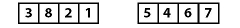
Let’s start with the following array:

And now we cut the array in half:
Now both of these arrays are cut in half repeatedly until each item is on its own:
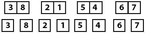
With the array now divided into the smallest possible parts, the process of merging those parts back together in sort-order occurs.
The individual items become sorted groups of two, those groups of two merge together into sorted groups of four, and then they finally all merge back together as a final sorted array.
Let’s take a moment to think about the individual operations that we need to implement:
- A way to split the arrays recursively. The
Sortmethod does this. - A way to merge the items together in sort-order. The
Mergemethod does this.
One performance consideration of the merge sort is that unlike the linear sorting algorithms, merge sort is going to perform its entire split and merge logic, including any memory allocations, even if the array is already in sorted order. While it has better worst-case performance than the linear sorting algorithms, its best-case performance will always be worse. This means it is not an ideal candidate when sorting data that is known to be nearly sorted; for example, when inserting data into an already sorted array.
public void Sort(T[] items)
{
	if (items.Length <= 1)
	{
		return;
	}

	int leftSize = items.Length / 2;
	int rightSize = items.Length - leftSize;

	T[] left = new T[leftSize];
	T[] right = new T[rightSize];

	Array.Copy(items, 0, left, 0, leftSize);
	Array.Copy(items, leftSize, right, 0, rightSize);

	Sort(left);
	Sort(right);
	Merge(items, left, right);
}

private void Merge(T[] items, T[] left, T[] right)
{
	int leftIndex = 0;
	int rightIndex = 0;
	int targetIndex = 0;

	int remaining = left.Length + right.Length;

	while(remaining > 0)
	{
		if (leftIndex >= left.Length)
		{
			items[targetIndex] = right[rightIndex++];
		}
		else if (rightIndex >= right.Length)
		{
			items[targetIndex] = left[leftIndex++];
		}
		else if (left[leftIndex].CompareTo(right[rightIndex]) < 0)
		{
			items[targetIndex] = left[leftIndex++];
		}
		else
		{
			items[targetIndex] = right[rightIndex++];
		}

		targetIndex++;
		remaining--;
	}
}
Quick Sort
| Behavior | Sorts the input array using the quick sort algorithm. | ||
| Complexity | Best Case | Average Case | Worst Case |
| Time | O(n log n) | O(n log n) | O(n2) |
| Space | O(1) | O(1) | O(1) |
Quick sort is another divide and conquer sorting algorithm. This one works by recursively performing the following algorithm:
- Pick a pivot index and partition the array into two arrays. This is done using a random number in the sample code. While there are other strategies, I favored a simple approach for this sample.
- Put all values less than the pivot value to the left of the pivot point and the values above the pivot value to the right. The pivot point is now sorted—everything to the right is larger; everything to the left is smaller. The value at the pivot point is in its correct sorted location.
- Repeat the pivot and partition algorithm on the unsorted left and right partitions until every item is in its known sorted position.
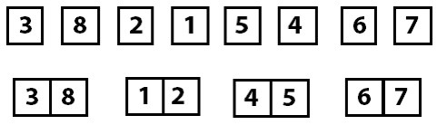
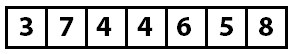
Let’s perform a quick sort on the following array:
Step one says we pick the partition point using a random index. In the sample code, this is done at this line:
int pivotIndex = _pivotRng.Next(left, right);
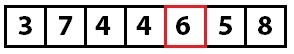
Now that we know the partition index (four), we look at the value at that point (six) and move the values in the array so that everything less than the value is on the left side of the array and everything else (values greater than or equal) is moved to the right side of the array. Keep in mind that moving the values around might change the index the partition value is stored at (we will see that shortly).
Swapping the values is done by the partition method in the sample code.
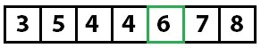
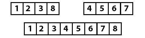
At this point, we know that six is in the correct spot in the array. We know this because every value to the left is less than the partition value, and everything to the right is greater than or equal to the partition value. Now we repeat this process on the two unsorted partitions of the array.
The repetition is done in the sample code by recursively calling the quicksort method with each of the array partitions. Notice that this time the left array is partitioned at index one with the value five. The process of moving the values to their appropriate positions moves the value five to another index. I point this out to reinforce the point that you are selecting a partition value, not a partition index.
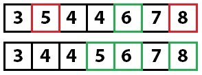
Quick sorting again:
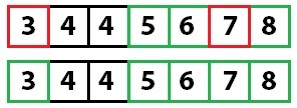
And quick sorting one last time:
With only one unsorted value left, and since we know that every other value is sorted, the array is fully sorted.
Random _pivotRng = new Random();

public void Sort(T[] items)
{
	quicksort(items, 0, items.Length - 1);
}

private void quicksort(T[] items, int left, int right)
{
	if (left < right)
	{
		int pivotIndex = _pivotRng.Next(left, right);
		int newPivot = partition(items, left, right, pivotIndex);

		quicksort(items, left, newPivot - 1);
		quicksort(items, newPivot + 1, right);
	}
}

private int partition(T[] items, int left, int right, int pivotIndex)
{
	T pivotValue = items[pivotIndex];

	Swap(items, pivotIndex, right);

	int storeIndex = left;

	for (int i = left; i < right; i++)
	{
		if (items[i].CompareTo(pivotValue) < 0)
		{
			Swap(items, i, storeIndex);
			storeIndex += 1;
		}
	}

	Swap(items, storeIndex, right);
	return storeIndex;
}

Comments